The 2025 World Rapid Chess Championship in New York is reaching its climax. After 9 grueling rounds of rapid chess, Magnus Carlsen sits on 7.0 points, chasing the leaders as the tournament enters its final stretch. With four rounds remaining (Rounds 10-13), the championship remains wide open.
In a 13-round Swiss tournament with over 200 players, predicting the winner is far more complex than a direct knockout. Players are paired based on their current score, meaning Magnus’s path to victory depends not just on his own results, but on how the entire field performs.
This analysis uses Monte Carlo simulation to answer the key question:
What are Magnus Carlsen’s chances of winning the World Rapid Championship, and how does his Round 10 result affect those odds?
The Challenge of Swiss System Tournaments
Unlike a round-robin or knockout format, Swiss system tournaments pair players with similar scores each round. This creates fascinating dynamics:
Leaders face each other: The top scorers are paired against each other, making it harder to maintain a lead
Half-point leads matter: In rapid chess with high draw rates, every half point is precious
Tiebreaks add complexity: Points alone may not determine the winner
For our simulation, we’ll focus on the primary criterion: final point total. Tiebreaks (Buchholz, Sonneborn-Berger, etc.) add another layer but require tracking every player’s full history.
Data Sources
We scrape live data from Chess-Results, the official tournament management system:
In Swiss tournaments, ties are common. Across our simulations:
79.4% of tournaments end with a sole winner
13.6% end in a 2-way tie
7.0% end in a 3+ way tie
Caveats and Limitations
This simulation has several important limitations:
Simulation Limitations
Approximate Swiss pairings: Rounds 11-13 use a simplified pairing algorithm that doesn’t enforce:
No repeat pairings
Strict color alternation
Full FIDE floating priorities
No tiebreaks: We only consider final point totals, not Buchholz, Sonneborn-Berger, or other tiebreak criteria
Static Elo model: Player form can vary significantly in rapid chess; we assume consistent performance
Top-80 focus: We simulate only the top 80 players by points/rating to keep computation tractable
Despite these limitations, the simulation provides valuable insight into the probability landscape heading into the tournament’s final day.
Conclusion
Monte Carlo simulation reveals the high-variance nature of Swiss system tournaments. Even with a relatively small number of rounds remaining, the uncertainty compounds across games and pairings.
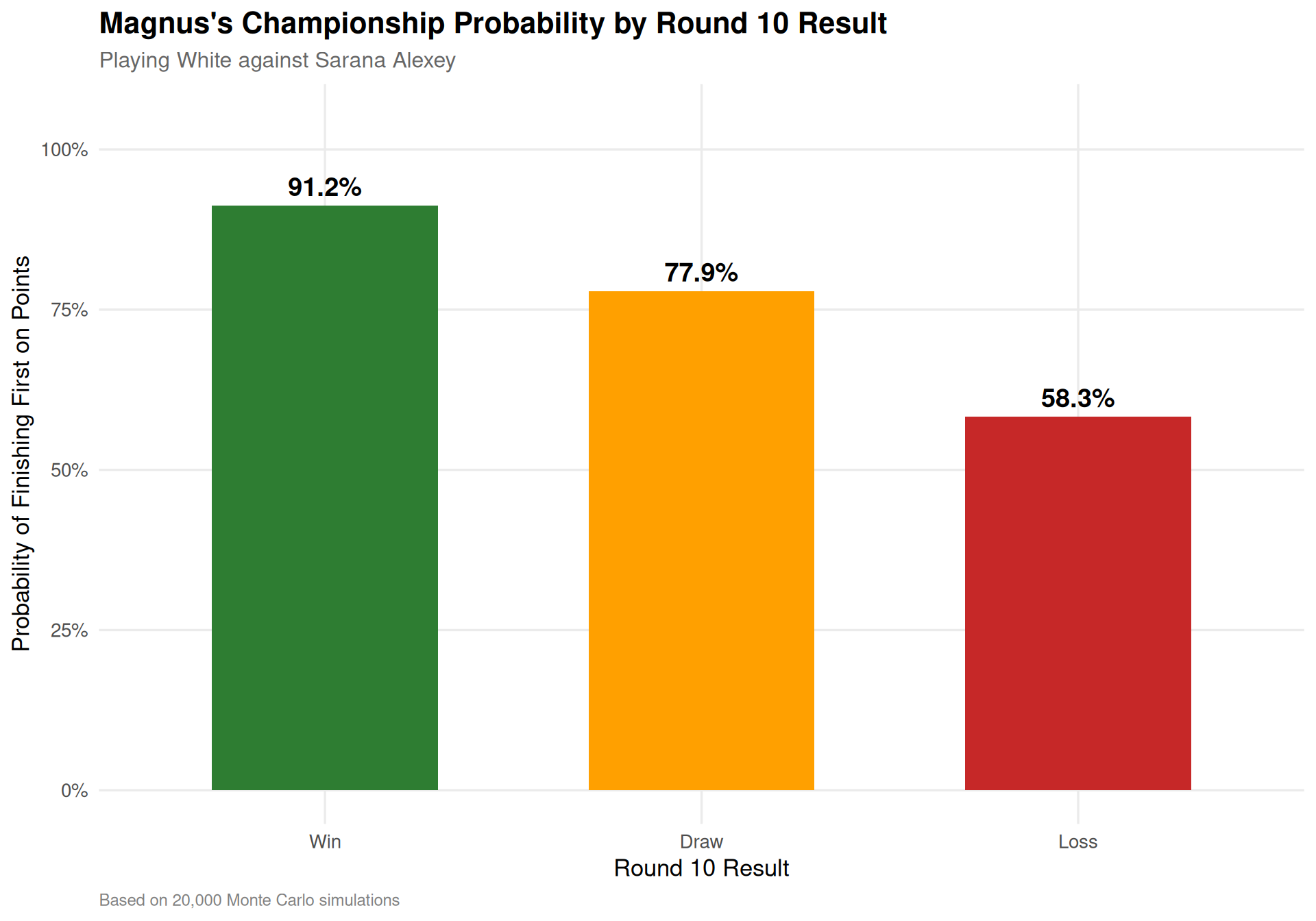
For Magnus Carlsen, the message is clear: Round 10 is crucial. A win would significantly boost his championship odds, while a loss would make an already challenging path considerably steeper.
The beauty of Swiss tournaments is that dramatic comebacks remain possible—but the mathematics of probability suggest Magnus needs to maximize his point total starting now.
Technical Notes
This analysis uses:
Python for Monte Carlo simulation and web scraping from Chess-Results
R/ggplot2 for data visualization
Quarto for reproducible polyglot data science
Reticulate for seamless Python-R integration
Data is scraped live from Chess-Results at render time.
Analysis current as of December 28, 2025, after Round 9 of the World Rapid Championship.
Source Code
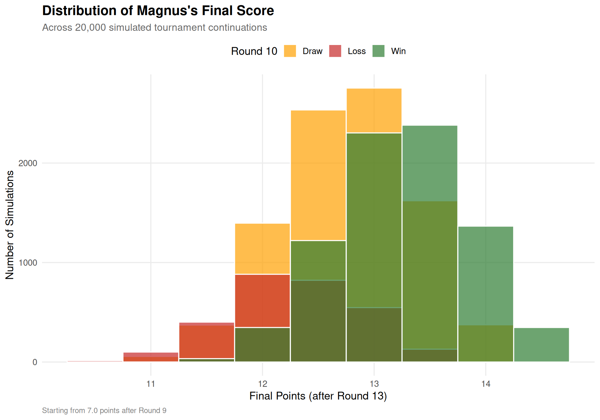
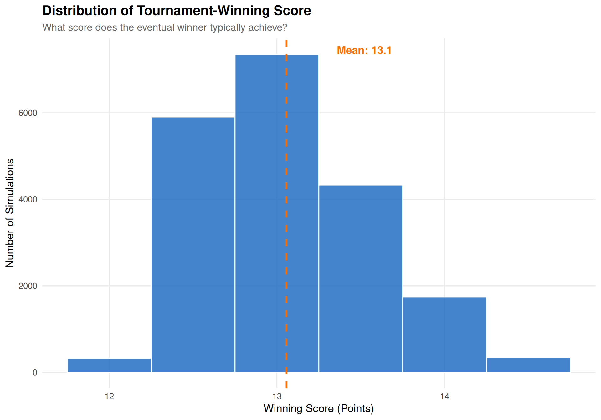
---title: "Can Magnus Carlsen Win the 2025 World Rapid Championship?"subtitle: "A Monte Carlo Simulation of the Final Four Rounds"author: "Kieran Mace"date: "2025-12-28"categories: [Python, R, Chess, Monte Carlo, Simulation]format: html: code-fold: true code-tools: true toc: true toc-depth: 3 fig-width: 10 fig-height: 7 theme: cosmoexecute: warning: false message: false---```{r setup}#| include: falselibrary(tidyverse)library(scales)library(viridis)library(reticulate)library(knitr)# Set ggplot2 themetheme_set(theme_minimal(base_size = 13) + theme( plot.title = element_text(face = "bold", size = 16), plot.subtitle = element_text(size = 12, color = "gray40"), plot.caption = element_text(size = 9, color = "gray50", hjust = 0), panel.grid.minor = element_blank(), legend.position = "right" ))```# IntroductionThe 2025 World Rapid Chess Championship in New York is reaching its climax. After 9 grueling rounds of rapid chess, **Magnus Carlsen** sits on **7.0 points**, chasing the leaders as the tournament enters its final stretch. With four rounds remaining (Rounds 10-13), the championship remains wide open.In a 13-round Swiss tournament with over 200 players, predicting the winner is far more complex than a direct knockout. Players are paired based on their current score, meaning Magnus's path to victory depends not just on his own results, but on how the entire field performs.This analysis uses **Monte Carlo simulation** to answer the key question:> **What are Magnus Carlsen's chances of winning the World Rapid Championship, and how does his Round 10 result affect those odds?**# The Challenge of Swiss System TournamentsUnlike a round-robin or knockout format, Swiss system tournaments pair players with similar scores each round. This creates fascinating dynamics:- **Leaders face each other**: The top scorers are paired against each other, making it harder to maintain a lead- **Half-point leads matter**: In rapid chess with high draw rates, every half point is precious- **Tiebreaks add complexity**: Points alone may not determine the winnerFor our simulation, we'll focus on the primary criterion: **final point total**. Tiebreaks (Buchholz, Sonneborn-Berger, etc.) add another layer but require tracking every player's full history.# Data SourcesWe scrape live data from [Chess-Results](https://chess-results.com), the official tournament management system:```{python}#| label: load-data#| echo: trueimport pandas as pdimport numpy as npfrom simulation import ( load_crosstable_after_rd9, load_round_pairings, outcome_probs, simulate_with_round10_outcome)# Load current standingsstandings = load_crosstable_after_rd9()# Load Round 10 pairingsrd10_pairings = load_round_pairings()# Find Magnus's pairingmagnus_pairing = rd10_pairings[ (rd10_pairings["white"] =="Carlsen Magnus") | (rd10_pairings["black"] =="Carlsen Magnus")]```## Current Standings (After Round 9)```{r}#| label: standings-tablestandings_r <- py$standings %>%head(15) %>%select(rank, name, rtg, pts) %>%rename(Rank = rank,Player = name,Rating = rtg,Points = pts )kable(standings_r, caption ="Top 15 players after Round 9")```## Round 10 Pairings (Published)```{r}#| label: pairings-table# Get top board pairingspairings_r <- py$rd10_pairings %>%head(10) %>%select(board, white, white_rtg, white_pts, black, black_rtg, black_pts) %>%rename(Board = board,White = white,`W.Rtg`= white_rtg,`W.Pts`= white_pts,Black = black,`B.Rtg`= black_rtg,`B.Pts`= black_pts )kable(pairings_r, caption ="Top 10 boards for Round 10")``````{python}#| label: magnus-opponent# Magnus's Round 10 opponentmagnus_row = magnus_pairing.iloc[0]if magnus_row["white"] =="Carlsen Magnus": magnus_color ="White" opponent_name = magnus_row["black"] opponent_rtg = magnus_row["black_rtg"]else: magnus_color ="Black" opponent_name = magnus_row["white"] opponent_rtg = magnus_row["white_rtg"]magnus_rtg = standings[standings["name"] =="Carlsen Magnus"]["rtg"].values[0]magnus_pts = standings[standings["name"] =="Carlsen Magnus"]["pts"].values[0]```:::{.callout-note appearance="simple"}## Magnus Carlsen's Round 10 Matchup**Magnus Carlsen** (`r sprintf("%.0f", py$magnus_rtg)`) plays **`r py$magnus_color`** against **`r py$opponent_name`** (`r sprintf("%.0f", py$opponent_rtg)`).Magnus is currently on **`r py$magnus_pts` points** after 9 rounds.:::# The Probability ModelFor each game, we use an **Elo-style probability model** with an adjustable draw rate. The model:1. Calculates expected score using the standard Elo formula2. Adjusts draw probability based on rating difference (closer ratings → more draws)3. Splits the remaining probability between wins for each player```{python}#| label: probability-demo#| echo: true# Example probabilities for Magnus vs his Round 10 opponentif magnus_color =="White": p_win, p_draw, p_loss = outcome_probs(magnus_rtg, opponent_rtg, draw_base=0.37)else: p_loss, p_draw, p_win = outcome_probs(opponent_rtg, magnus_rtg, draw_base=0.37)prob_display = pd.DataFrame({"Outcome": ["Magnus Wins", "Draw", "Magnus Loses"],"Probability": [f"{p_win:.1%}", f"{p_draw:.1%}", f"{p_loss:.1%}"]})``````{r}#| label: prob-tablekable(py$prob_display, caption ="Round 10 outcome probabilities for Magnus")```The `draw_base` parameter is set to 0.37, reflecting the higher draw rates typical in rapid chess at the elite level.# Monte Carlo SimulationWe simulate the remaining 4 rounds (10-13) across **20,000 possible futures**:- **Round 10**: Uses the published pairings from Chess-Results- **Rounds 11-13**: Uses an approximate Swiss pairing algorithm (score groups + rating sort)```{python}#| label: run-simulation#| echo: true# Run simulation with Round 10 outcome trackingresults = simulate_with_round10_outcome( n_sims=20000, seed=42, focus_top_n=80, draw_base=0.37, focus_player="Carlsen Magnus")# Overall championship probabilityoverall_prob = results["focus_is_co_winner"].mean()# Conditional probabilities by Round 10 outcomecond_probs = results.groupby("focus_rd10_outcome").agg({"focus_is_co_winner": ["mean", "count"]}).reset_index()cond_probs.columns = ["Round 10 Result", "Championship Prob", "N Simulations"]cond_probs = cond_probs.sort_values("Championship Prob", ascending=False)```# Results## Overall Championship Probability```{r}#| label: overall-proboverall <- py$overall_prob```Based on 20,000 simulated tournament continuations, **Magnus Carlsen has a `r sprintf("%.1f%%", py$overall_prob * 100)` chance** of finishing first (or tied for first) on points.## How Round 10 Affects Magnus's Chances```{r}#| label: fig-conditional-prob#| fig-cap: "Magnus's championship probability conditional on his Round 10 result. A win dramatically improves his odds."cond_data <- py$cond_probs %>%mutate(`Round 10 Result`=factor(`Round 10 Result`, levels =c("Win", "Draw", "Loss")) )ggplot(cond_data, aes(x =`Round 10 Result`, y =`Championship Prob`, fill =`Round 10 Result`)) +geom_col(width =0.6) +geom_text(aes(label =sprintf("%.1f%%", `Championship Prob`*100)),vjust =-0.5, size =5, fontface ="bold") +scale_y_continuous(labels = percent, limits =c(0, max(cond_data$`Championship Prob`) *1.15)) +scale_fill_manual(values =c("Win"="#2E7D32", "Draw"="#FFA000", "Loss"="#C62828")) +labs(title ="Magnus's Championship Probability by Round 10 Result",subtitle =sprintf("Playing %s against %s", py$magnus_color, py$opponent_name),x ="Round 10 Result",y ="Probability of Finishing First on Points",caption ="Based on 20,000 Monte Carlo simulations" ) +theme(legend.position ="none")``````{r}#| label: conditional-tablekable( cond_data %>%mutate(`Championship Prob`=sprintf("%.1f%%", `Championship Prob`*100),`N Simulations`=format(`N Simulations`, big.mark =",") ),caption ="Championship probability by Round 10 outcome")```## Distribution of Final Scores```{r}#| label: fig-score-distribution#| fig-cap: "Distribution of Magnus's final score across all simulations, colored by Round 10 result."results_r <- py$resultsggplot(results_r, aes(x = focus_pts, fill = focus_rd10_outcome)) +geom_histogram(binwidth =0.5, position ="identity", alpha =0.7, color ="white") +scale_fill_manual(values =c("Win"="#2E7D32", "Draw"="#FFA000", "Loss"="#C62828"),name ="Round 10" ) +labs(title ="Distribution of Magnus's Final Score",subtitle ="Across 20,000 simulated tournament continuations",x ="Final Points (after Round 13)",y ="Number of Simulations",caption ="Starting from 7.0 points after Round 9" ) +theme(legend.position ="top")``````{r}#| label: score-statsscore_summary <- results_r %>%group_by(focus_rd10_outcome) %>%summarise(`Mean Score`=mean(focus_pts),`Median Score`=median(focus_pts),`Min Score`=min(focus_pts),`Max Score`=max(focus_pts),.groups ="drop" ) %>%rename(`Round 10`= focus_rd10_outcome) %>%arrange(desc(`Mean Score`))kable(score_summary, digits =2, caption ="Summary statistics for Magnus's final score")```## Winning Score AnalysisWhat score is needed to win this tournament?```{r}#| label: fig-winning-scores#| fig-cap: "Distribution of the winning score across all simulations. The tournament appears to require around 10-11 points to win."ggplot(results_r, aes(x = max_pts)) +geom_histogram(binwidth =0.5, fill ="#1565C0", color ="white", alpha =0.8) +geom_vline(aes(xintercept =mean(max_pts)), color ="#FF6F00", linetype ="dashed", linewidth =1) +annotate("text", x =mean(results_r$max_pts) +0.3, y =Inf,label =sprintf("Mean: %.1f", mean(results_r$max_pts)),vjust =2, hjust =0, color ="#FF6F00", fontface ="bold") +labs(title ="Distribution of Tournament-Winning Score",subtitle ="What score does the eventual winner typically achieve?",x ="Winning Score (Points)",y ="Number of Simulations" )```## Ties for First Place```{r}#| label: tie-analysistie_stats <- results_r %>%summarise(`Sole Winner`=mean(n_tied ==1),`2-Way Tie`=mean(n_tied ==2),`3+ Way Tie`=mean(n_tied >=3) )```In Swiss tournaments, ties are common. Across our simulations:- **`r sprintf("%.1f%%", tie_stats[["Sole Winner"]] * 100)`** of tournaments end with a sole winner- **`r sprintf("%.1f%%", tie_stats[["2-Way Tie"]] * 100)`** end in a 2-way tie- **`r sprintf("%.1f%%", tie_stats[["3+ Way Tie"]] * 100)`** end in a 3+ way tie# Caveats and LimitationsThis simulation has several important limitations::::{.callout-warning}## Simulation Limitations1. **Approximate Swiss pairings**: Rounds 11-13 use a simplified pairing algorithm that doesn't enforce: - No repeat pairings - Strict color alternation - Full FIDE floating priorities2. **No tiebreaks**: We only consider final point totals, not Buchholz, Sonneborn-Berger, or other tiebreak criteria3. **Static Elo model**: Player form can vary significantly in rapid chess; we assume consistent performance4. **Top-80 focus**: We simulate only the top 80 players by points/rating to keep computation tractable:::Despite these limitations, the simulation provides valuable insight into the probability landscape heading into the tournament's final day.# ConclusionMonte Carlo simulation reveals the high-variance nature of Swiss system tournaments. Even with a relatively small number of rounds remaining, the uncertainty compounds across games and pairings.For Magnus Carlsen, the message is clear: **Round 10 is crucial**. A win would significantly boost his championship odds, while a loss would make an already challenging path considerably steeper.The beauty of Swiss tournaments is that dramatic comebacks remain possible—but the mathematics of probability suggest Magnus needs to maximize his point total starting now.:::{.callout-tip}## Technical NotesThis analysis uses:- **Python** for Monte Carlo simulation and web scraping from Chess-Results- **R/ggplot2** for data visualization- **Quarto** for reproducible polyglot data science- **Reticulate** for seamless Python-R integrationData is scraped live from [Chess-Results](https://chess-results.com) at render time.:::---*Analysis current as of December 28, 2025, after Round 9 of the World Rapid Championship.*