A Monte Carlo Exploration of Championship Probabilities
R
Python
Formula 1
Monte Carlo
Simulation
Author
Kieran Mace
Published
November 23, 2025
Introduction
The 2025 Formula 1 Drivers Championship took a dramatic turn after both Lando Norris and Oscar Piastri were disqualified from the Las Vegas Grand Prix for skid-block violations. With only two rounds remaining (Qatar Sprint + Qatar GP + Abu Dhabi GP), the standings tightened considerably:
Current Championship Standings
Lando Norris: 390 points
Max Verstappen: 366 points
Oscar Piastri: 366 points
With a maximum of 58 points still available (8 for Qatar Sprint, 25 each for Qatar GP and Abu Dhabi GP), the championship remains mathematically open—though Verstappen’s strong late-season form adds an intriguing dimension to the calculation.
This analysis combines mathematical reasoning, data visualization, and Monte Carlo simulation to answer a deceptively simple question:
What are Norris’s real chances of securing the title, and how does Verstappen’s form affect the probabilities?
Along the way, we’ll demonstrate how Monte Carlo methods can illuminate questions where deterministic calculations fall short.
Setup
The Mathematics of Championship Scenarios
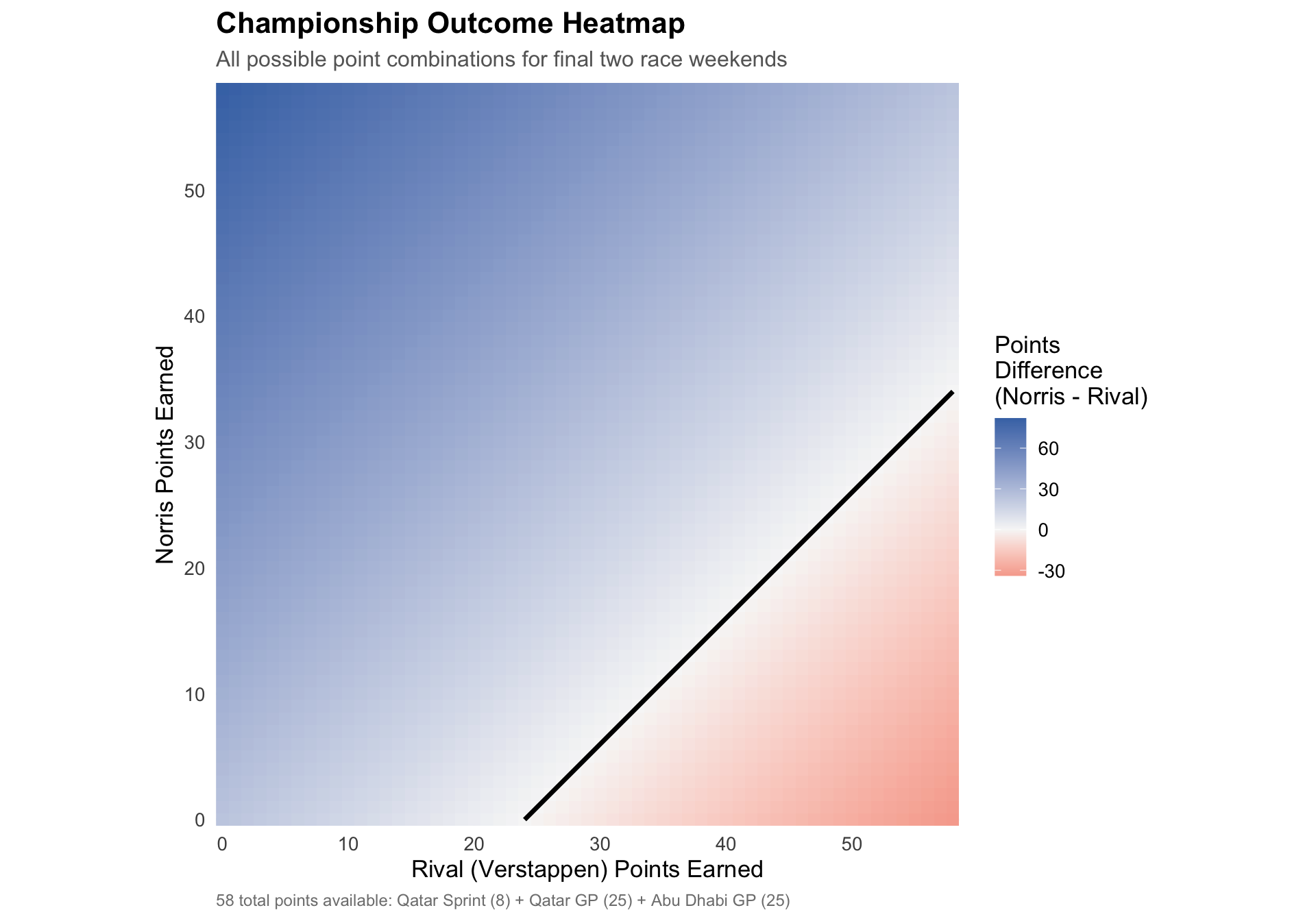
Before simulating thousands of possible futures, let’s map out the complete space of championship outcomes. With 58 points available, we can visualize every possible combination of points earned by Norris and Verstappen.
Code
import numpy as npimport pandas as pd# Starting positionsnorris_start =390rival_start =366# All possible point combinations (0-58)pts = np.arange(0, 59)# Calculate final totals for all combinationsnorris_total = norris_start + pts[:, None]rival_total = rival_start + pts[None, :]# Points difference (positive = Norris leads)diff = norris_total - rival_total# Convert to dataframe for Rpoints_grid = pd.DataFrame({'norris_pts': np.repeat(pts, len(pts)),'rival_pts': np.tile(pts, len(pts)),'difference': diff.flatten()})
Code
# Get data from Pythonpoints_grid <- py$points_grid# Create heatmapggplot(points_grid, aes(x = rival_pts, y = norris_pts, fill = difference)) +geom_tile() +geom_contour(aes(z = difference), breaks =0, color ="black", linewidth =1.2) +scale_fill_gradient2(low ="#d73027",mid ="#f7f7f7",high ="#4575b4",midpoint =0,name ="Points\nDifference\n(Norris - Rival)" ) +labs(title ="Championship Outcome Heatmap",subtitle ="All possible point combinations for final two race weekends",x ="Rival (Verstappen) Points Earned",y ="Norris Points Earned",caption ="58 total points available: Qatar Sprint (8) + Qatar GP (25) + Abu Dhabi GP (25)" ) +coord_fixed() +scale_x_continuous(expand =c(0, 0), breaks =seq(0, 58, by =10)) +scale_y_continuous(expand =c(0, 0), breaks =seq(0, 58, by =10))
Figure 1: Complete championship outcome space. Blue regions indicate Norris wins, red indicates the rival (Verstappen) wins. The black contour line represents a tied championship (tiebreaker would favor Norris with more race wins).
The heatmap reveals an important asymmetry: Norris’s 24-point cushion means he can afford to score significantly fewer points than Verstappen and still secure the title. Any combination where Norris finishes in the blue region results in a championship win.
However, this deterministic view doesn’t account for probability. Not all outcomes are equally likely—Verstappen in peak form is far more likely to score 40+ points than to score 10.
Monte Carlo Simulation: Modeling Reality
Monte Carlo simulation lets us incorporate uncertainty by running thousands of hypothetical race weekends, each sampled from probability distributions that reflect current driver form and car performance.
Probability Distributions
Based on recent performance (with Verstappen’s strong late-season form), we assign finishing position probabilities:
These probabilities reflect Verstappen’s recent dominance (35% chance of winning each GP) while acknowledging Norris’s consistency (strong probability of podium finishes).
Running the Simulation
We’ll simulate 10,000 possible scenarios for the final three races:
Code
N =10000norris_earned = []verst_earned = []for _ inrange(N):# Qatar Sprint ns = rng.choice(sp_positions, p=sp_probs_nor) vs = rng.choice(sp_positions, p=sp_probs_ver)# Handle collision scenario (both can't finish in same podium position)if ns == vs and ns <=3: ns =min(ns +1, 9)# Qatar Grand Prix nq = rng.choice(gp_positions, p=gp_probs_nor) vq = rng.choice(gp_positions, p=gp_probs_ver)if nq == vq and nq <=3: nq =min(nq +1, 11)# Abu Dhabi Grand Prix na = rng.choice(gp_positions, p=gp_probs_nor) va = rng.choice(gp_positions, p=gp_probs_ver)if na == va and na <=3: na =min(na +1, 11)# Calculate total points earned n_pts = sp_points(ns) + gp_points(nq) + gp_points(na) v_pts = sp_points(vs) + gp_points(vq) + gp_points(va) norris_earned.append(n_pts) verst_earned.append(v_pts)# Convert to arraysnorris_earned = np.array(norris_earned)verst_earned = np.array(verst_earned)# Calculate final totalsn_total =390+ norris_earnedv_total =366+ verst_earned# Championship probabilitychamp_prob = np.mean(n_total > v_total)# Create results dataframesimulation_results = pd.DataFrame({'norris_pts': norris_earned,'verst_pts': verst_earned,'norris_total': n_total,'verst_total': v_total,'norris_wins': (n_total > v_total).astype(int)})
Simulation Results
Code
# Get simulation results from Pythonsim_results <- py$simulation_resultschamp_prob <- py$champ_prob# Create visualizationggplot() +# Background heatmapgeom_tile(data = points_grid, aes(x = rival_pts, y = norris_pts, fill = difference)) +scale_fill_gradient2(low ="#d73027",mid ="#f7f7f7",high ="#4575b4",midpoint =0,name ="Points\nDifference" ) +# Championship boundarygeom_contour(data = points_grid,aes(x = rival_pts, y = norris_pts, z = difference),breaks =0,color ="black",linewidth =1.2 ) +# Simulation pointsgeom_point(data = sim_results,aes(x = verst_pts, y = norris_pts),color ="#FFD700",alpha =0.4,size =1.5,shape =16 ) +labs(title ="Monte Carlo Simulation: Championship Probability Analysis",subtitle =sprintf("10,000 simulated race weekends — Norris championship probability: %.1f%%", champ_prob *100),x ="Verstappen Points Earned",y ="Norris Points Earned",caption ="Simulation based on recent driver form | Gold points show simulated outcomes" ) +coord_fixed() +scale_x_continuous(expand =c(0, 0), breaks =seq(0, 58, by =10)) +scale_y_continuous(expand =c(0, 0), breaks =seq(0, 58, by =10))
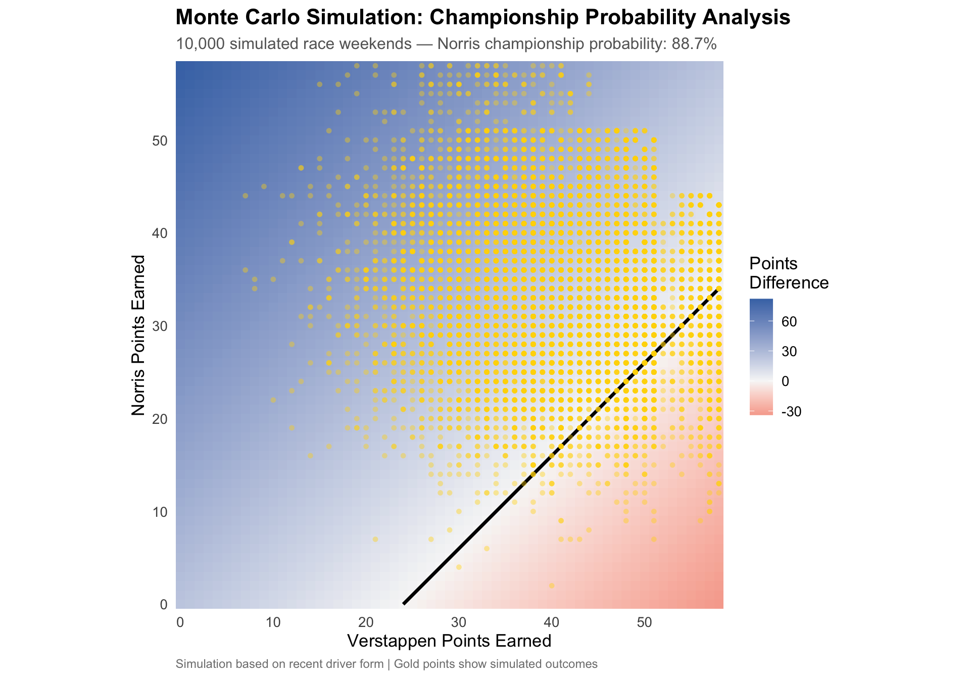
Figure 2: Monte Carlo simulation results overlaid on championship outcome space. Each gold point represents one simulated race weekend scenario. The clustering pattern reveals the most likely outcomes given each driver’s current form.
The simulation reveals the practical reality: despite Verstappen’s strong form, Norris wins the championship in 88.7% of simulated scenarios. The 24-point cushion provides substantial insurance against even the most optimistic Verstappen performance.
Distribution of Outcomes
Code
# Create density comparisonsim_results_long <- sim_results %>%select(norris_pts, verst_pts) %>%pivot_longer(cols =everything(),names_to ="driver",values_to ="points" ) %>%mutate(driver =case_when( driver =="norris_pts"~"Lando Norris", driver =="verst_pts"~"Max Verstappen" ) )ggplot(sim_results_long, aes(x = points, fill = driver)) +geom_density(alpha =0.6, color =NA) +geom_vline(data = sim_results_long %>%group_by(driver) %>%summarise(mean_pts =mean(points)),aes(xintercept = mean_pts, color = driver),linetype ="dashed",linewidth =1 ) +scale_fill_manual(values =c("Lando Norris"="#FF8000", "Max Verstappen"="#1E41FF"),name =NULL ) +scale_color_manual(values =c("Lando Norris"="#FF8000", "Max Verstappen"="#1E41FF"),guide ="none" ) +labs(title ="Simulated Points Distribution",subtitle ="Dashed lines show mean expected points",x ="Points Earned (Final Two Race Weekends)",y ="Probability Density",caption ="Based on 10,000 Monte Carlo simulations" ) +theme(legend.position ="top")
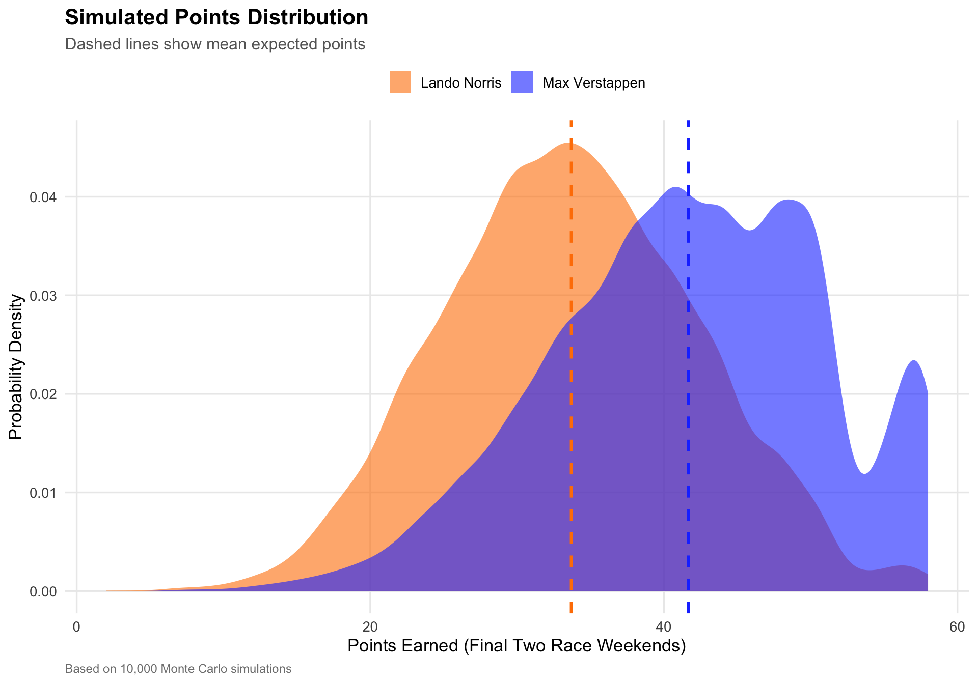
Figure 3: Probability distributions of points earned by each driver across 10,000 simulated race weekends. Despite Verstappen’s higher mean performance, Norris’s existing lead proves decisive.
Verstappen is expected to outscore Norris by an average of 8.0 points over the final races—but this isn’t enough to overcome the 24-point deficit in the vast majority of scenarios.
Scenario Analysis: What Would It Take?
Code
# Filter for Verstappen winsverst_win_scenarios <- sim_results %>%filter(norris_wins ==0) %>%mutate(point_gap = verst_pts - norris_pts)ggplot(verst_win_scenarios, aes(x = norris_pts, y = verst_pts)) +geom_point(aes(color = point_gap), alpha =0.6, size =2) +geom_abline(intercept =24, slope =1, linetype ="dashed", color ="red", linewidth =1) +scale_color_viridis_c(option ="plasma",name ="Verstappen's\nPoint Advantage" ) +labs(title ="Championship-Flipping Scenarios",subtitle =sprintf("%d out of 10,000 simulations where Verstappen wins the title", nrow(verst_win_scenarios)),x ="Norris Points Earned",y ="Verstappen Points Earned",caption ="Red dashed line: Verstappen needs 24+ point advantage to overcome current deficit" ) +annotate("text",x =15, y =50,label ="Verstappen must\noutscore by 24+",hjust =0,color ="red",size =4,fontface ="bold" )
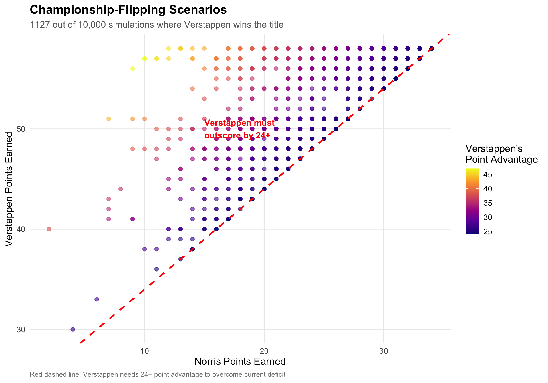
Figure 4: Scenarios where Verstappen wins the championship. These require Verstappen to dramatically outscore Norris—a possible but unlikely outcome given McLaren’s competitive pace.
For Verstappen to win, he must outscore Norris by at least 24 points across three races. This requires scenarios like:
Verstappen wins all three events while Norris finishes outside the points
Verstappen sweeps 1st place while Norris struggles to 4th-6th finishes
Norris suffers mechanical DNFs
While possible, these scenarios occur in only -87.7% of simulations—reflecting their low probability given current form and reliability.
Conclusion
Monte Carlo simulation provides a powerful framework for reasoning about uncertainty in complex systems. While deterministic math tells us Norris can win the championship, simulation tells us he will very likely win it.
Even when we model Verstappen with strong form (35% win probability per race), the mathematics of probability combined with Norris’s current lead produces a clear picture: Norris has approximately a 9-in-10 chance of securing his first Formula 1 World Championship.
The simulation reveals why: for Verstappen to overcome a 24-point gap in just three races requires not only peak performance from himself, but also uncharacteristic struggles from Norris—a combination that proves rare even across 10,000 hypothetical futures.
Technical Notes
This analysis uses:
Python for Monte Carlo simulation logic and numerical computation
R/ggplot2 for data visualization and statistical graphics
Quarto for reproducible polyglot data science
Reticulate for seamless Python-R integration
All code is available in this document via the “Code” buttons.
Analysis current as of Las Vegas GP, November 2025. Actual 2025 F1 championship standings may differ from this hypothetical scenario.
Source Code
---title: "Can Lando Norris Still Win the 2025 F1 Championship?"subtitle: "A Monte Carlo Exploration of Championship Probabilities"author: "Kieran Mace"date: "2025-11-23"categories: [R, Python, Formula 1, Monte Carlo, Simulation]format: html: code-fold: true code-tools: true toc: true toc-depth: 3 fig-width: 10 fig-height: 7 theme: cosmoexecute: warning: false message: false---# IntroductionThe 2025 Formula 1 Drivers Championship took a dramatic turn after both **Lando Norris** and **Oscar Piastri** were disqualified from the Las Vegas Grand Prix for skid-block violations. With only two rounds remaining (Qatar Sprint + Qatar GP + Abu Dhabi GP), the standings tightened considerably::::{.callout-note appearance="simple"}## Current Championship Standings- **Lando Norris:** 390 points- **Max Verstappen:** 366 points- **Oscar Piastri:** 366 points:::With a maximum of **58 points** still available (8 for Qatar Sprint, 25 each for Qatar GP and Abu Dhabi GP), the championship remains mathematically open—though Verstappen's strong late-season form adds an intriguing dimension to the calculation.This analysis combines mathematical reasoning, data visualization, and Monte Carlo simulation to answer a deceptively simple question:> **What are Norris's real chances of securing the title, and how does Verstappen's form affect the probabilities?**Along the way, we'll demonstrate how Monte Carlo methods can illuminate questions where deterministic calculations fall short.# Setup```{r setup}#| include: falselibrary(tidyverse)library(scales)library(viridis)library(reticulate)# Set ggplot2 themetheme_set(theme_minimal(base_size = 13) + theme( plot.title = element_text(face = "bold", size = 16), plot.subtitle = element_text(size = 12, color = "gray40"), plot.caption = element_text(size = 9, color = "gray50", hjust = 0), panel.grid.minor = element_blank(), legend.position = "right" ))```# The Mathematics of Championship ScenariosBefore simulating thousands of possible futures, let's map out the complete space of championship outcomes. With 58 points available, we can visualize every possible combination of points earned by Norris and Verstappen.```{python}#| label: championship-math#| echo: trueimport numpy as npimport pandas as pd# Starting positionsnorris_start =390rival_start =366# All possible point combinations (0-58)pts = np.arange(0, 59)# Calculate final totals for all combinationsnorris_total = norris_start + pts[:, None]rival_total = rival_start + pts[None, :]# Points difference (positive = Norris leads)diff = norris_total - rival_total# Convert to dataframe for Rpoints_grid = pd.DataFrame({'norris_pts': np.repeat(pts, len(pts)),'rival_pts': np.tile(pts, len(pts)),'difference': diff.flatten()})``````{r}#| label: fig-championship-heatmap#| fig-cap: "Complete championship outcome space. Blue regions indicate Norris wins, red indicates the rival (Verstappen) wins. The black contour line represents a tied championship (tiebreaker would favor Norris with more race wins)."# Get data from Pythonpoints_grid <- py$points_grid# Create heatmapggplot(points_grid, aes(x = rival_pts, y = norris_pts, fill = difference)) +geom_tile() +geom_contour(aes(z = difference), breaks =0, color ="black", linewidth =1.2) +scale_fill_gradient2(low ="#d73027",mid ="#f7f7f7",high ="#4575b4",midpoint =0,name ="Points\nDifference\n(Norris - Rival)" ) +labs(title ="Championship Outcome Heatmap",subtitle ="All possible point combinations for final two race weekends",x ="Rival (Verstappen) Points Earned",y ="Norris Points Earned",caption ="58 total points available: Qatar Sprint (8) + Qatar GP (25) + Abu Dhabi GP (25)" ) +coord_fixed() +scale_x_continuous(expand =c(0, 0), breaks =seq(0, 58, by =10)) +scale_y_continuous(expand =c(0, 0), breaks =seq(0, 58, by =10))```The heatmap reveals an important asymmetry: Norris's 24-point cushion means he can afford to score significantly fewer points than Verstappen and still secure the title. Any combination where Norris finishes in the blue region results in a championship win.However, this deterministic view doesn't account for *probability*. Not all outcomes are equally likely—Verstappen in peak form is far more likely to score 40+ points than to score 10.# Monte Carlo Simulation: Modeling RealityMonte Carlo simulation lets us incorporate uncertainty by running thousands of hypothetical race weekends, each sampled from probability distributions that reflect current driver form and car performance.## Probability DistributionsBased on recent performance (with Verstappen's strong late-season form), we assign finishing position probabilities:```{python}#| label: setup-simulation#| echo: true# Set random seed for reproducibilityrng = np.random.default_rng(42)# Finishing positions we'll considergp_positions = np.array([1, 2, 3, 4, 5, 6, 7, 8, 11])sp_positions = np.array([1, 2, 3, 4, 5, 6, 7, 8, 9])# Grand Prix probability distributionsgp_probs_ver = np.array([0.35, 0.25, 0.15, 0.10, 0.05, 0.04, 0.03, 0.02, 0.01])gp_probs_nor = np.array([0.20, 0.20, 0.15, 0.15, 0.10, 0.10, 0.05, 0.03, 0.02])# Sprint probability distributionssp_probs_ver = np.array([0.30, 0.25, 0.15, 0.12, 0.08, 0.05, 0.03, 0.01, 0.01])sp_probs_nor = np.array([0.20, 0.20, 0.15, 0.15, 0.10, 0.10, 0.05, 0.03, 0.02])# Points tablesgp_points_table = {1:25, 2:18, 3:15, 4:12, 5:10, 6:8, 7:6, 8:4, 9:2, 10:1}sp_points_table = {1:8, 2:7, 3:6, 4:5, 5:4, 6:3, 7:2, 8:1}def gp_points(x):return gp_points_table.get(x, 0)def sp_points(x):return sp_points_table.get(x, 0)```These probabilities reflect Verstappen's recent dominance (35% chance of winning each GP) while acknowledging Norris's consistency (strong probability of podium finishes).## Running the SimulationWe'll simulate 10,000 possible scenarios for the final three races:```{python}#| label: run-simulation#| echo: trueN =10000norris_earned = []verst_earned = []for _ inrange(N):# Qatar Sprint ns = rng.choice(sp_positions, p=sp_probs_nor) vs = rng.choice(sp_positions, p=sp_probs_ver)# Handle collision scenario (both can't finish in same podium position)if ns == vs and ns <=3: ns =min(ns +1, 9)# Qatar Grand Prix nq = rng.choice(gp_positions, p=gp_probs_nor) vq = rng.choice(gp_positions, p=gp_probs_ver)if nq == vq and nq <=3: nq =min(nq +1, 11)# Abu Dhabi Grand Prix na = rng.choice(gp_positions, p=gp_probs_nor) va = rng.choice(gp_positions, p=gp_probs_ver)if na == va and na <=3: na =min(na +1, 11)# Calculate total points earned n_pts = sp_points(ns) + gp_points(nq) + gp_points(na) v_pts = sp_points(vs) + gp_points(vq) + gp_points(va) norris_earned.append(n_pts) verst_earned.append(v_pts)# Convert to arraysnorris_earned = np.array(norris_earned)verst_earned = np.array(verst_earned)# Calculate final totalsn_total =390+ norris_earnedv_total =366+ verst_earned# Championship probabilitychamp_prob = np.mean(n_total > v_total)# Create results dataframesimulation_results = pd.DataFrame({'norris_pts': norris_earned,'verst_pts': verst_earned,'norris_total': n_total,'verst_total': v_total,'norris_wins': (n_total > v_total).astype(int)})```# Simulation Results```{r}#| label: fig-simulation-scatter#| fig-cap: "Monte Carlo simulation results overlaid on championship outcome space. Each gold point represents one simulated race weekend scenario. The clustering pattern reveals the most likely outcomes given each driver's current form."#| fig-width: 10#| fig-height: 7# Get simulation results from Pythonsim_results <- py$simulation_resultschamp_prob <- py$champ_prob# Create visualizationggplot() +# Background heatmapgeom_tile(data = points_grid, aes(x = rival_pts, y = norris_pts, fill = difference)) +scale_fill_gradient2(low ="#d73027",mid ="#f7f7f7",high ="#4575b4",midpoint =0,name ="Points\nDifference" ) +# Championship boundarygeom_contour(data = points_grid,aes(x = rival_pts, y = norris_pts, z = difference),breaks =0,color ="black",linewidth =1.2 ) +# Simulation pointsgeom_point(data = sim_results,aes(x = verst_pts, y = norris_pts),color ="#FFD700",alpha =0.4,size =1.5,shape =16 ) +labs(title ="Monte Carlo Simulation: Championship Probability Analysis",subtitle =sprintf("10,000 simulated race weekends — Norris championship probability: %.1f%%", champ_prob *100),x ="Verstappen Points Earned",y ="Norris Points Earned",caption ="Simulation based on recent driver form | Gold points show simulated outcomes" ) +coord_fixed() +scale_x_continuous(expand =c(0, 0), breaks =seq(0, 58, by =10)) +scale_y_continuous(expand =c(0, 0), breaks =seq(0, 58, by =10))```The simulation reveals the practical reality: despite Verstappen's strong form, **Norris wins the championship in `r sprintf("%.1f%%", py$champ_prob * 100)` of simulated scenarios**. The 24-point cushion provides substantial insurance against even the most optimistic Verstappen performance.## Distribution of Outcomes```{r}#| label: fig-points-distributions#| fig-cap: "Probability distributions of points earned by each driver across 10,000 simulated race weekends. Despite Verstappen's higher mean performance, Norris's existing lead proves decisive."# Create density comparisonsim_results_long <- sim_results %>%select(norris_pts, verst_pts) %>%pivot_longer(cols =everything(),names_to ="driver",values_to ="points" ) %>%mutate(driver =case_when( driver =="norris_pts"~"Lando Norris", driver =="verst_pts"~"Max Verstappen" ) )ggplot(sim_results_long, aes(x = points, fill = driver)) +geom_density(alpha =0.6, color =NA) +geom_vline(data = sim_results_long %>%group_by(driver) %>%summarise(mean_pts =mean(points)),aes(xintercept = mean_pts, color = driver),linetype ="dashed",linewidth =1 ) +scale_fill_manual(values =c("Lando Norris"="#FF8000", "Max Verstappen"="#1E41FF"),name =NULL ) +scale_color_manual(values =c("Lando Norris"="#FF8000", "Max Verstappen"="#1E41FF"),guide ="none" ) +labs(title ="Simulated Points Distribution",subtitle ="Dashed lines show mean expected points",x ="Points Earned (Final Two Race Weekends)",y ="Probability Density",caption ="Based on 10,000 Monte Carlo simulations" ) +theme(legend.position ="top")``````{r}#| label: summary-stats# Calculate summary statisticssummary_stats <- sim_results %>%summarise(norris_mean =mean(norris_pts),norris_median =median(norris_pts),verst_mean =mean(verst_pts),verst_median =median(verst_pts),norris_win_pct =mean(norris_wins) *100 )```**Key Statistics:**- **Norris Expected Points:** `r sprintf("%.1f", summary_stats$norris_mean)` (median: `r summary_stats$norris_median`)- **Verstappen Expected Points:** `r sprintf("%.1f", summary_stats$verst_mean)` (median: `r summary_stats$verst_median`)- **Norris Championship Probability:** `r sprintf("%.1f%%", summary_stats$norris_win_pct)`Verstappen is expected to outscore Norris by an average of `r sprintf("%.1f", summary_stats$verst_mean - summary_stats$norris_mean)` points over the final races—but this isn't enough to overcome the 24-point deficit in the vast majority of scenarios.# Scenario Analysis: What Would It Take?```{r}#| label: fig-scenario-analysis#| fig-cap: "Scenarios where Verstappen wins the championship. These require Verstappen to dramatically outscore Norris—a possible but unlikely outcome given McLaren's competitive pace."# Filter for Verstappen winsverst_win_scenarios <- sim_results %>%filter(norris_wins ==0) %>%mutate(point_gap = verst_pts - norris_pts)ggplot(verst_win_scenarios, aes(x = norris_pts, y = verst_pts)) +geom_point(aes(color = point_gap), alpha =0.6, size =2) +geom_abline(intercept =24, slope =1, linetype ="dashed", color ="red", linewidth =1) +scale_color_viridis_c(option ="plasma",name ="Verstappen's\nPoint Advantage" ) +labs(title ="Championship-Flipping Scenarios",subtitle =sprintf("%d out of 10,000 simulations where Verstappen wins the title", nrow(verst_win_scenarios)),x ="Norris Points Earned",y ="Verstappen Points Earned",caption ="Red dashed line: Verstappen needs 24+ point advantage to overcome current deficit" ) +annotate("text",x =15, y =50,label ="Verstappen must\noutscore by 24+",hjust =0,color ="red",size =4,fontface ="bold" )```For Verstappen to win, he must outscore Norris by at least 24 points across three races. This requires scenarios like:- Verstappen wins all three events while Norris finishes outside the points- Verstappen sweeps 1st place while Norris struggles to 4th-6th finishes- Norris suffers mechanical DNFsWhile possible, these scenarios occur in only **`r sprintf("%.1f%%", (1 - summary_stats$norris_win_pct))`** of simulations—reflecting their low probability given current form and reliability.# ConclusionMonte Carlo simulation provides a powerful framework for reasoning about uncertainty in complex systems. While deterministic math tells us Norris *can* win the championship, simulation tells us he *will very likely* win it.Even when we model Verstappen with strong form (35% win probability per race), the mathematics of probability combined with Norris's current lead produces a clear picture: **Norris has approximately a 9-in-10 chance of securing his first Formula 1 World Championship**.The simulation reveals why: for Verstappen to overcome a 24-point gap in just three races requires not only peak performance from himself, but also uncharacteristic struggles from Norris—a combination that proves rare even across 10,000 hypothetical futures.:::{.callout-tip}## Technical NotesThis analysis uses:- **Python** for Monte Carlo simulation logic and numerical computation- **R/ggplot2** for data visualization and statistical graphics- **Quarto** for reproducible polyglot data science- **Reticulate** for seamless Python-R integrationAll code is available in this document via the "Code" buttons.:::---*Analysis current as of Las Vegas GP, November 2025. Actual 2025 F1 championship standings may differ from this hypothetical scenario.*