Exploring Homoscedasticity in Gene Expression

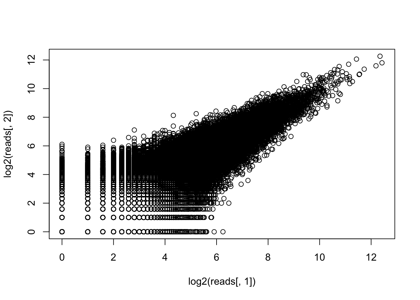
library(DESeq2)
dds <- makeExampleDESeqDataSet(n=50000,m=4)
reads = counts(dds)
plot(log2(reads[,1]),log2(reads[,2]))

reads_mean = apply(reads,1,mean)
reads_sd = apply(reads,1, sd)
plot(reads_mean, reads_sd)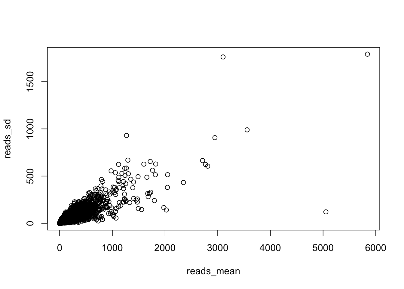

Now lets normalize library size and esimate dispersion:

dds = estimateSizeFactors(dds)
#estimateDispersions(dds)
ntd = assay(normTransform(dds)) # regular log2 with a psudocount
rld = assay(rlog(dds)) # doing the same thing as log2, but not allowing low counts to explode 

library("vsn")
meanSdPlot(ntd, ranks=F)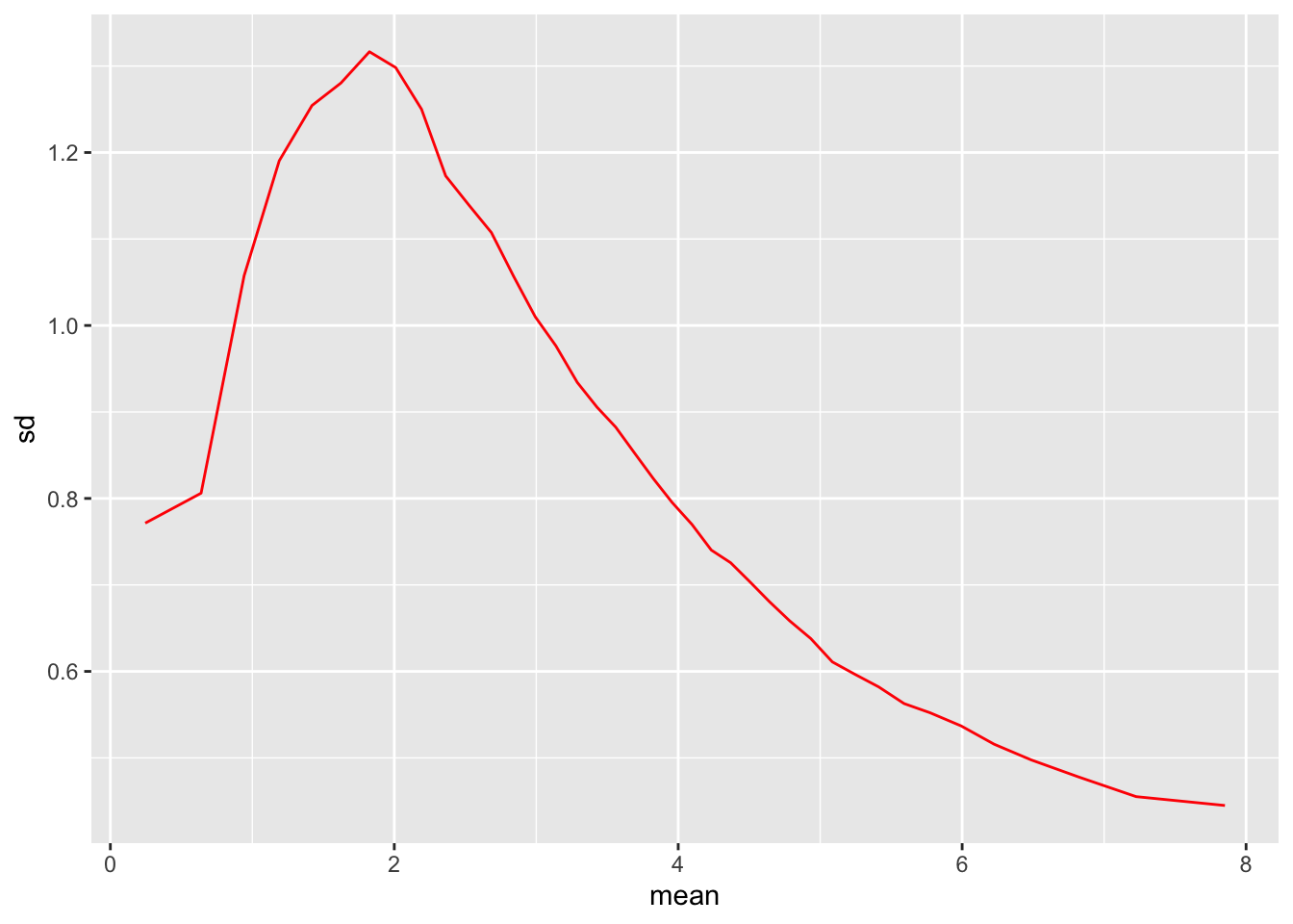

meanSdPlot(rld, ranks=F)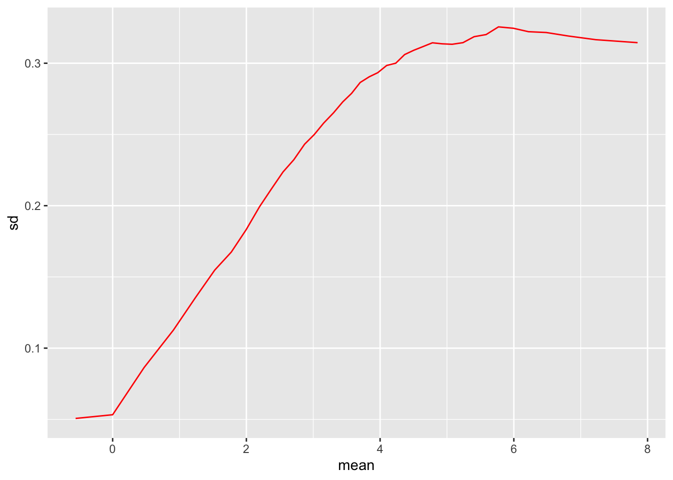

So here we can see that we have shrunk the sd at low levels

plot(rld[,1],rld[,2])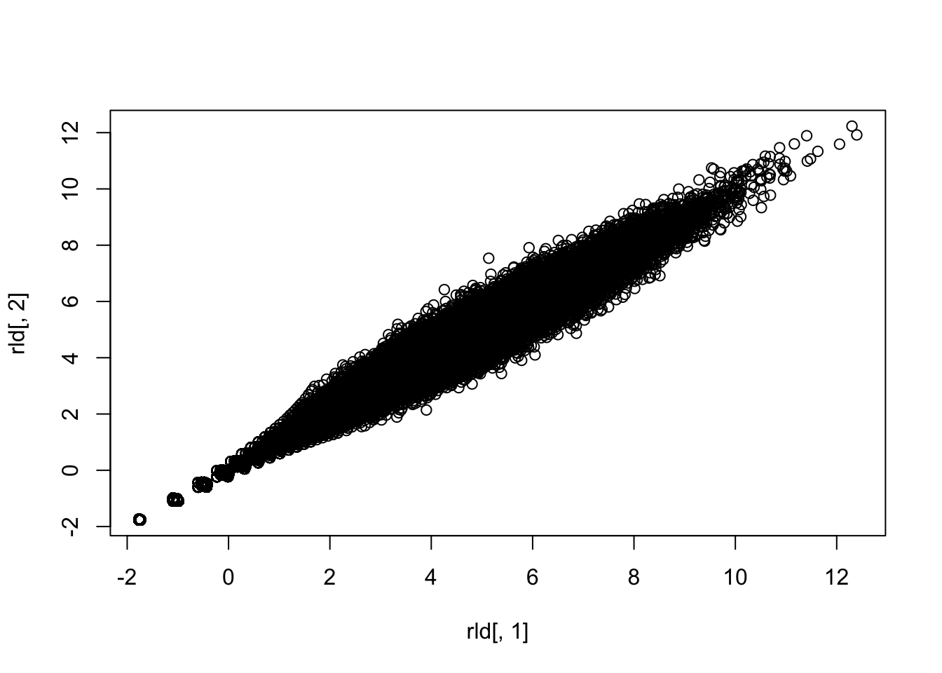

now lets do it ourselves:

ntd_mean = apply(ntd,1,mean)
ntd_sd = apply(ntd,1,sd)
plot(ntd_mean,ntd_sd)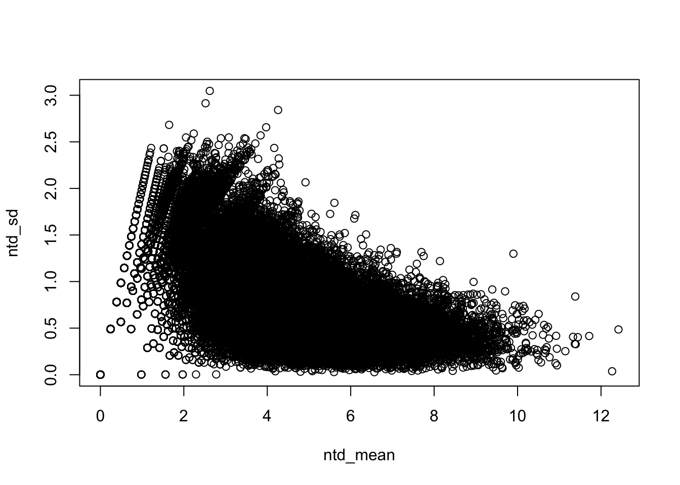

library(mgcv)
model <- smooth.spline(ntd_mean, ntd_sd) # build the model
fit <- predict( model , se = TRUE )$fit # estimated values
se <- predict( model , se = TRUE)$se.fit # standard error

# Confidence interval:
lcl <- fit - 1.96 * se
ucl <- fit + 1.96 * se


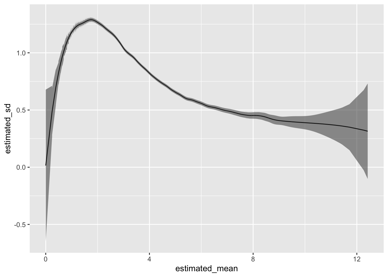
fit <- smooth.spline(ntd_mean, ntd_sd)      # smooth.spline fit
res <- (fit$yin - fit$y)/(1-fit$lev)      # jackknife residuals
sigma <- sqrt(var(res))                     # estimate sd

upper <- fit$y + 2.0*sigma*sqrt(fit$lev)   # upper 95% conf. band
lower <- fit$y - 2.0*sigma*sqrt(fit$lev) 

data = data.frame(estimated_mean = fit$x,
                  estimated_sd = fit$y,
                  lower_bound = lower,
                  upper_bound = upper)

library(ggplot2)

ggplot(data) +
       geom_line(aes(x = estimated_mean,
                     y = estimated_sd)) + 
       geom_ribbon(aes(x = estimated_mean,
                       ymax = upper_bound,
                       ymin = lower_bound), alpha=0.5)